Implementing Efficient Graph Based Image Segmentation with C++

This is a summary and my implementation of the research paper Efficient Graph based Image Segmentation. To understand the implementation it is recommended to know C++ (pointers, vectors, structs, linked lists, pass by reference and return by reference).

What is Image Segmentation?

Image Segmentation is the process of dividing an image into sementaic regions, where each region represents a separate object. Quoting wikipedia:

More precisely, image segmentation is the process of assigning a label to every pixel in an image such that pixels with the same label share certain characteristics.

Look at the following examples:

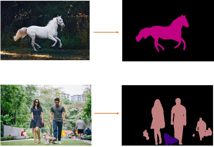
Source - https://www.learnopencv.com/applications-of-foreground-background-separation-with-semantic-segmentation/

Now this might be a very trivial task for the human brain, but no so easy for the computer.

There have been a good number of methods in the past to solve this problem but either they were not convincing or efficient enough for larger adoption and real world applications. In 2004, Pedro F. Felzenszwalb (MIT) and Daniel P. Huttenlocher (Cornell), published this method to be more effective and efficient compared to previous methods for this problem. We are going to discuss this method in this article.

What this particular method aims to achieve?

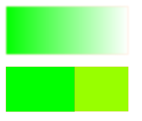
Extract global aspects of an image – this means grouping and dividing all regions which are perceptually important. They achieve this based on a predicate that measures the evidence of a boundary. As the algorithm states,

Intuitively, the intensity differences across the boundary of two regions are perceptually important if they are large relative to the intensity differences inside at least one of the regions.

You can see in the top rectangle that it is only one region even if there is an entire white space at the right hand side of the box. In the second rectangle, there are clearly two regions due to the boundary at the center. The regions are perceptually important.

Be super fast. To be of practical use, the segmentation needs to be as quick as edge detection techniques or could be run at several frames per second (important for any video applications)

Defining the Graph

\[G = (V, E)\]

The graph G is an undirected weighted graph with vertices $v_i \in V$ and edges $(v_i, v_j) \in E$ corresponding to pairs of adjacent vertices. In this context, the vertices represent the pixels of the image.

Each region, also called as the Component, will be denoted by $C$, i.e., $C_1, C_2, \dots C_k$ are componets from Component 1 to Component k.

The edges of the graph can be weighted using intensity differences of two pixels. If it’s a grayscale image the the weight of an edge between vertices $v_i$ and $v_j$ can be calculated using:

\[w(e_{ij}) = |I_i - I_j|\]

where $I_i$ and $I_j$ are intensities of vertex $v_i$ and $v_j$ respectively.

If you want differences between rgb pixels:

\[w(e_{ij}) = \sqrt{ (r_i - r_j)^2 + (b_i - b_j)^2 + (g_i - g_j)^2}\]

where $r_p$, $b_p$ and $g_p$ are intensities of red, blue and green channels of the vertex p, respectively.

Defining the metrics to measure a boundary between regions

The algorithm merges any two Componets(regions) if there is no evidence for a bounday between them. And how is this evidence measured? Well there are 4 simple equations to understand:

First we need to know the differences within a region:

\[Int(C) = \max_{e \in MST(C, E)} w(e)\]

Int(C) is the internal difference of a component C defined as the maximum edge of the Minimum Spanning Tree (MST) of the component C. MST is calculated using the Kruskal’s algorithm. For those who want a refresher on MST, can find a simple and intuitive explanation here.

Then we need to find differences between the regions:

\[Dif(C_1,C_2) = \min_{v_i \in C_1, v_j \in C_2, (v_i, v_j) \in E} w((v_i, v_j))\]

The Difference between two components is meased by the minimum of the weighted edges connecting the two components.

We also need a thresholding function that controls the degree of how much the internal difference of two regions should be lower than the difference between the regions to conclude there is an evidence for a boundary.

\[\Gamma(C) = k/|C|\]

Here k is constant, which controls the degree of difference required between internal and external differences to find a boundary. $ | C | $ is the size of the component which is equal to the number of pixels in the component.

In my opinion, we need this thresholding to confidently divide or merge two regions and also be more robust against high-variability regions.

Finally, the algorithm evaluates the evidence of a boundary by checking if the difference between components is larger than the internal difference of any of the two components. Which means, there is a boundary between two components if Dif(C_1, C_2) should be greater than the minimum of the internal difference of the two components.

\[MInt(C_1, C_2) = min(Int(C_1) + k/|C_1|, Int(C_2) + k/|C_2|)\]

Of course, if the second component is large, the value of $\Gamma$ would be comparatively low and increases the possibilities of merging the two components. That also emphasizes the point that larger k prefers larger components.

and the final equation is:

\[\begin{equation} D(C_1, C_2) = \begin{cases} true &\text{if $Dif(C_1, C_2) > MInt(C_1, C_2)$}\\ false &\text{othersie} \end{cases} \end{equation}\]

To conclude, the above equation means that there is evidence of a boundary if the external difference between two components is greater than the internal difference of any of the components relative to there size ($k/|C|$).

The Algorithm

We start with the initial setup where each pixel is its own componets and $Int(C) = 0$, as $|C| = 1$ (no edges).

Sort the edges in non-decreasing order
Loop through each edge

For the $qth$ iteration, $v_i$ and $v_j$ are the vertices connected to the $qth$ edge in the ordering, i.e., $e_q = (v_i, v_j)$ and belong to components $C_i$ and $C_j$ respectively. If $v_i$ and $v_j$ are in different components ($C_i \neq C_j$) and $MInt(C_i, C_j)$ > $Dif(C_i, C_j)$ then merge the components, otherwise do nothing.

That’s it. That’s the algorithm. Pretty simple eh?

Intuition

Larger k causes a preference for larger components(components with more pixels).

Consider k = 700 and the range of intensities is [0, 255]. In this case, the size of resulting components will be at least 3 pixels. This is because if range is [0, 255] then the maximum weight (difference between two pixels) is also 255. Let S be a component of size 3, then:
\[\Gamma(S) = 700/3\] \[\Gamma(S) \approx 233\]
This means that for the component S to have a boundary with another component P(let $|P| = 2$ and $Int(P) > Int(S)$) , it’s internal difference should be at least 233 units less than the minimum edge connecting 2 components. And if component S was of size 10, then $\Gamma = 70$. A comparatively smaller difference between external and internal differences is required to merge components. So with lower components size a higher difference is required(stronger evidence) to prove existence of a boundary, which means that the component is likely to be merged and merging of two components results in a larger component.
You can take any other measures as weight.

In place of intensity differences, you can take other measures for weight such as location of pixels, HSV color space values, motion, or other attributes. Anything that works for your use-case.
Threshold function can also be modified to identify particular shapes

You can also change the threshold function such that it identifies particular shapes such as circles, squares or pretty much anything. In this case, not all segmentations will be of this particular shape but one of two neighboring regions will be of this particular shape.

Implementation

You can access my entire Github Repo for the most recent updates.

Here’s my cmake file:

cmake_minimum_required(VERSION 3.16)
project(GraphBasedImageSegmentation)

set(CMAKE_CXX_STANDARD 17)
find_package(OpenCV REQUIRED)
add_executable(GraphBasedImageSegmentation main.cpp DisjointForest.cpp utils.cpp segmentation.cpp)

include_directories(${OpenCV_INCLUDE_DIRS})
target_link_libraries(GraphBasedImageSegmentation PUBLIC ${OpenCV_LIBS})

I have used a Disjoint Forest to represent our segmentation as suggested by the paper. To summarize disjoint Forest Data Structure:

It is a faster implementation of the Disjoint Set Data Stucture. A disjoint set is a collections of sets which do not have any elements in common. A Disjoint Set uses linked lists to represent sets whereas a disjoint forest uses trees. In our case, each set(tree) represents a component and each element of a component represents a unique pixel.
Each set has a representative, like an identity to identify a unique set. In our case, the representative of a component is the first pixel of the component(or the root node of the tree).
Merging two sets results in a single set whose size is equal to the sum of the two merged sets. In our case, we merge two sets when we find a evidence for a boundary between them (when $D(C_i, C_j)$ is true).

DisjointForest.h

#pragma once
#include <vector>
#include <functional>
#include <memory>
#include <opencv2/opencv.hpp>

struct Component;
struct ComponentStruct;
struct Pixel;
struct Edge;

using component_pointer = std::shared_ptr<Component>;
using component_struct_pointer = std::shared_ptr<ComponentStruct>;
using pixel_pointer = std::shared_ptr<Pixel>;
using edge_pointer = std::shared_ptr<Edge>;

struct Pixel{
    component_pointer parentTree;
    pixel_pointer parent;
    int intensity;
    int bValue;
    int gValue;
    int rValue;
    int row;
    int column;
};

struct Component{
    component_struct_pointer parentComponentStruct;
    std::vector<pixel_pointer> pixels;
    int rank = 0;
    pixel_pointer representative;
    double MSTMaxEdge = 0;
};

struct Edge{
    double weight;
    pixel_pointer n1;
    pixel_pointer n2;
};

struct ComponentStruct{
    component_struct_pointer previousComponentStruct=nullptr;
    component_pointer component{};
    component_struct_pointer nextComponentStruct= nullptr;
};

edge_pointer createEdge(const pixel_pointer& pixel1, const pixel_pointer& pixel2, const std::function<double(pixel_pointer , pixel_pointer)>& edgeDifferenceFunction);
double rgbPixelDifference(const pixel_pointer& pixel1, const pixel_pointer& pixel2);
double grayPixelDifference(const pixel_pointer& pixel1, const pixel_pointer& pixel2);
void mergeComponents(const component_pointer& x, const component_pointer& y, double MSTMaxEdgeValue);
component_pointer makeComponent(int row, int column, const cv::Vec3b& pixelValues);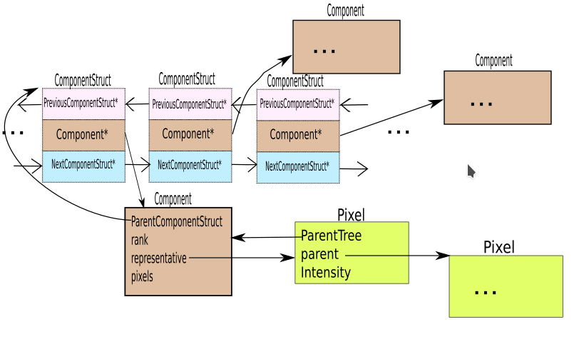

Each component is pointed by an element of a linked list which is represented by ComponentStruct. This linked list is necessary to remember the resulting components through out the program.

Explanation

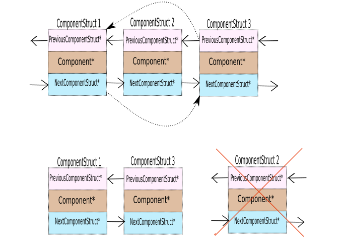
Each ComponentStruct also represents a component in a linked list. It points to the previous ComponentStruct and the next ComponentStruct in the linked list. Each time two components are merged, one ComponentStruct is deleted and the adjacent neighboring ComponentStructs in the list point to one another.
A component has a vector of pixels and a representative. The representative is initiated as the first pixel of the component. The component also points to the ComponentStruct in the linked list which points to the component. The rank represents the height of the component(The component is a tree structure). When two components are merged the component with lower rank is merged into the component with higher rank.
Each Pixel represents an individual pixel of the image that needs to be segmented. It holds its itensity, location((row, column)) and the component it belongs too.

DisjointForest.cpp

#include "DisjointForest.h"
#include <cmath>


std::shared_ptr<Component> makeComponent(const int row, const int column, const cv::Vec3b& pixelValues){
    std::shared_ptr<Component> component = std::make_shared<Component>();
    std::shared_ptr<Pixel> pixel = std::make_shared<Pixel>();
    pixel->bValue = pixelValues.val[0];
    pixel->gValue = pixelValues.val[1];
    pixel->rValue = pixelValues.val[2];
    pixel->intensity = (pixelValues.val[0] + pixelValues.val[1] + pixelValues.val[2])/3;
    pixel->row = row;
    pixel->column = column;
    pixel->parent = static_cast<std::shared_ptr<Pixel>>(pixel);
    pixel->parentTree = static_cast<std::shared_ptr<Component>>(component);
    component->representative = static_cast<std::shared_ptr<Pixel>>(pixel);
    component->pixels.push_back(std::move(pixel));
    return component;
}

void setParentTree(const component_pointer& childTreePointer, const component_pointer& parentTreePointer){
    for(const auto& nodePointer: childTreePointer->pixels){
        parentTreePointer->pixels.push_back(nodePointer);
        nodePointer->parentTree = parentTreePointer;
    }
}

double grayPixelDifference(const pixel_pointer &pixel1, const pixel_pointer& pixel2) {
    return abs(pixel1->intensity - pixel2->intensity);
}

double rgbPixelDifference(const pixel_pointer& pixel1, const pixel_pointer& pixel2){
    return sqrt(pow(pixel1->rValue- pixel2->rValue, 2 ) +
                pow(pixel1->bValue- pixel2->bValue, 2) +
                pow(pixel1->gValue- pixel2->gValue, 2));
}

edge_pointer createEdge(const pixel_pointer& pixel1, const pixel_pointer& pixel2, const std::function<double(pixel_pointer, pixel_pointer)> &edgeDifferenceFunction){
    edge_pointer edge = std::make_shared<Edge>();
    edge->weight = edgeDifferenceFunction(pixel1, pixel2);
    edge->n1 = pixel1;
    edge->n2 = pixel2;
    return edge;
}

void mergeComponents(const component_pointer& x, const component_pointer& y, const double MSTMaxEdgeValue){
    if (x != y) {
        component_struct_pointer componentStruct;
        if (x->rank < y->rank) {
            x->representative->parent = y->representative;
            y->MSTMaxEdge = MSTMaxEdgeValue;
            setParentTree(x, y);
            componentStruct = x->parentComponentStruct;
        } else {
            if (x->rank == y->rank) {
                ++x->rank;
            }
            y->representative->parent = x->representative->parent;
            x->MSTMaxEdge = MSTMaxEdgeValue;
            setParentTree(y, x);
            componentStruct = y->parentComponentStruct;
        }
        if(componentStruct->previousComponentStruct){
            componentStruct->previousComponentStruct->nextComponentStruct = componentStruct->nextComponentStruct;
        }
        if(componentStruct->nextComponentStruct){
            componentStruct->nextComponentStruct->previousComponentStruct = componentStruct->previousComponentStruct;
        }
    }
}

Explanation:

makeComponent creates a component with a single element(pixel). As you will see in utils.cpp, that initially each pixel is part of a separate component.
createEdge creates an Edge object using two Pixel Object pointers and sets weight depending on the colorSpace given. If we are comparing rgb differences then edgeDifferenceFunction is rgbPixelDifference euclidean difference of rgb values) otherwise it is grayPixelDifference(absolute difference between the pixel intensities).
mergeComponents has multi-fold operations. If Component A is merged into Component B (rank(A) < rank(B)):
- Sets A’s representative parent as B’s representative.
- Add’s all the pixels A to the pixels of the component B
- Deletes the componentStruct of A and points the previousComponentStruct and nextComponentStruct accordingly.

When ComponentStruct 2 is deleted, the ComponentStruct 1 points to ComponentStruct 3 as it's nextComponentStruct and ComponentStruct 1 points to ComponentStruct 3 as its previousComponentStruct.

utils.h

int getSingleIndex(int row, int col, int totalColumns);
int getEdgeArraySize(int rows, int columns);
std::vector<edge_pointer> setEdges(const std::vector<pixel_pointer> &pixels, std::string colorSpace, int rows, int columns);
cv::Mat addColorToSegmentation(component_struct_pointer componentStruct, int rows, int columns);
std::string getFileNameFromPath(const std::string &path);
void printParameters(const std::string &inputPath, const std::string &outputDir, const std::string &color,
                     float sigma, float k, int minimumComponentSize);
std::vector<pixel_pointer> constructImagePixels(const cv::Mat &img, int rows, int columns);

utils.cpp

#include <string>
#include <iostream>
#include <functional>
#include <vector>
#include <cstdlib>
#include <opencv2/opencv.hpp>
#include "DisjointForest.h"


int getSingleIndex(const int row, const int col, const int totalColumns){
    return (row*totalColumns) + col;
}

void printParameters(const std::string &inputPath, const std::string &outputDir, const std::string &color,
        const float sigma, const float k, const int minimumComponentSize){
    std::cout << "Input Path: " << inputPath << '\n';
    std::cout << "Output Directory: " << outputDir << '\n';
    std::cout << "Color Space: " << color << '\n';
    std::cout << "Sigma: " << sigma << '\n';
    std::cout << "k: " << k << '\n';
    std::cout << "Minimum Component Size: " << minimumComponentSize << '\n';
}

std::vector<std::string> split(const std::string& s, const char separator)
{
    std::vector<std::string> output;
    std::string::size_type prev_pos = 0, pos = 0;
    while((pos = s.find(separator, pos)) != std::string::npos)
    {
        std::string substring( s.substr(prev_pos, pos-prev_pos) );
        output.push_back(substring);
        prev_pos = ++pos;
    }
    output.push_back(s.substr(prev_pos, pos-prev_pos)); // Last word
    return output;
}

std::string getFileNameFromPath(const std::string &path){
    std::vector<std::string> pathSplit = split(path, '/');
    std::string fileName = pathSplit[pathSplit.size()-1];
    std::vector<std::string> fileNameSplit = split(fileName, '.');
    std::string baseFileName = fileNameSplit[0];
    return baseFileName;
}

int getEdgeArraySize(const int rows,const int columns){
    int firstColumn = 3 * (rows-1);
    int lastColumn = 2 * (rows - 1);
    int middleValues = 4 * (rows - 1 ) * (columns - 2);
    int lastRow = columns - 1;
    return firstColumn + lastColumn + middleValues + lastRow;
}

std::vector<pixel_pointer> constructImagePixels(const cv::Mat &img, int rows, int columns){
    std::vector<pixel_pointer> pixels(rows*columns);

    component_pointer firstComponent = makeComponent(0, 0, img.at<cv::Vec3b>(0, 0));
    component_struct_pointer firstComponentStruct =std::make_shared<ComponentStruct>();
    firstComponentStruct->component = firstComponent;
    auto previousComponentStruct = firstComponentStruct;
    int index;

    for(int row=0; row < rows; row++)
    {
        for(int column=0; column < columns; column++)
        {
            component_pointer component=makeComponent(row, column, img.at<cv::Vec3b>(row, column));
            component_struct_pointer newComponentStruct = std::make_shared<ComponentStruct>();
            newComponentStruct->component = component;
            newComponentStruct->previousComponentStruct = previousComponentStruct;
            previousComponentStruct->nextComponentStruct = newComponentStruct;
            component->parentComponentStruct = newComponentStruct;
            previousComponentStruct = newComponentStruct;
            index = getSingleIndex(row, column, columns);
            pixels[index] = component->pixels.at(0);
        }
    }
    firstComponentStruct = firstComponentStruct->nextComponentStruct;
    firstComponentStruct->previousComponentStruct = nullptr;
    return pixels;
}

std::vector<edge_pointer> setEdges(const std::vector<pixel_pointer> &pixels, const std::string colorSpace, const int rows, const int columns){
    int edgeArraySize = getEdgeArraySize(rows, columns);
    std::vector<edge_pointer> edges(edgeArraySize);
    std::function<double(pixel_pointer, pixel_pointer)> edgeDifferenceFunction;
    if (colorSpace == "rgb"){
        edgeDifferenceFunction = rgbPixelDifference;
    }else{
        edgeDifferenceFunction = grayPixelDifference;
    }
    int edgeCount = 0;
    for(int row=0; row < rows; ++row){
        for(int column=0; column < columns; ++column) {
            pixel_pointer presentPixel = pixels[getSingleIndex(row, column, columns)];
            if(row < rows - 1){
                if(column == 0){
                    edges[edgeCount++] = createEdge(presentPixel, pixels[getSingleIndex(row, column+1, columns)], edgeDifferenceFunction);
                    edges[edgeCount++] = createEdge(presentPixel, pixels[getSingleIndex(row+1, column+1, columns)], edgeDifferenceFunction);
                    edges[edgeCount++] = createEdge(presentPixel , pixels[getSingleIndex(row+1, column, columns)], edgeDifferenceFunction);
                }
                else if(column==columns-1){
                    edges[edgeCount++] = createEdge(presentPixel, pixels[getSingleIndex(row+1, column, columns)], edgeDifferenceFunction);
                    edges[edgeCount++] = createEdge(presentPixel, pixels[getSingleIndex(row+1, column-1, columns)], edgeDifferenceFunction);
                }else{
                    edges[edgeCount++] = createEdge(presentPixel, pixels[getSingleIndex(row, column+1, columns)], edgeDifferenceFunction);
                    edges[edgeCount++] = createEdge(presentPixel, pixels[getSingleIndex(row+1, column+1, columns)], edgeDifferenceFunction);
                    edges[edgeCount++] = createEdge(presentPixel, pixels[getSingleIndex(row+1, column, columns)], edgeDifferenceFunction);
                    edges[edgeCount++] = createEdge(presentPixel, pixels[getSingleIndex(row+1, column-1, columns)], edgeDifferenceFunction);
                }
            }
            else if(row == rows - 1){
                if(column != columns - 1) {
                    edges[edgeCount++] = createEdge(presentPixel, pixels[getSingleIndex(row,column+1, columns)], edgeDifferenceFunction);
                }
            }
        }
    }
    std::cout << "Total Edges: "<< edgeCount << '\n';
    return edges;
}

int getRandomNumber(const int min,const int max)
{
    //from learncpp.com
    static constexpr double fraction { 1.0 / (RAND_MAX + 1.0) };
    return min + static_cast<int>((max - min + 1) * (std::rand() * fraction));
}

cv::Mat addColorToSegmentation(component_struct_pointer componentStruct, const int rows, const int columns){
    cv::Mat segmentedImage(rows, columns, CV_8UC3);
    do{
        uchar r=getRandomNumber(0, 255);
        uchar b=getRandomNumber(0, 255);
        uchar g=getRandomNumber(0, 255);
        cv::Vec3b pixelColor= {b ,g ,r};
        for(const auto& pixel: componentStruct->component->pixels){
            segmentedImage.at<cv::Vec3b>(cv::Point(pixel->column,pixel->row)) = pixelColor;
        }
        componentStruct = componentStruct->nextComponentStruct;
    }while(componentStruct);
    
    return segmentedImage;
}

Explanation

constructImageGraph constructs the linked list while creating components and pixels. This function is initiating the graph, by creating a component for each pixel and adding a component to the linkedlist. Note that the pixels vector is one dimensional. So a getSingleIndex is used to get the corresponding index where the pixel needs to be saved/accessed based on its location(row & column) in the image.
addColorToSegmentation adds color to all the componentStruct(Remember that ComponentStruct is pointing a single Component). All pixels of a component are assigned a single random color
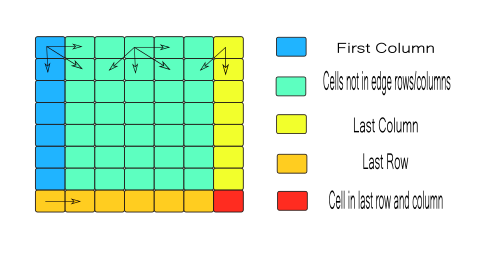
setEdges creates edges as displayed by the image below:

The above image shows which neighbors are considered for each category of pixels to compute pixel differences(edge weights). For example, the pixels in blue category(first column except last row) will only compute differences with right neighbor, bottom neighbor and right-diagonal neighbor. Using these categories, all neighboring pixel intensity differences(edge weights) are captured and are calculated only once.

segmentation.h

void segmentImage(const std::vector<edge_pointer> &edges, int totalComponents, int minimumComponentSize, float kValue);

segmentation.cpp

#include <iostream>
#include <vector>
#include "DisjointForest.h"

inline float thresholdFunction(const float componentSize,const float k){
    return k/componentSize;
}

void segmentImage(const std::vector<edge_pointer> &edges, int totalComponents, const int minimumComponentSize, const float kValue) {
    std::cout << "Starting Segmentation:\n";
    pixel_pointer pixel1;
    pixel_pointer pixel2;
    component_pointer component1;
    component_pointer component2;
    double minimumInternalDifference;
    for(const auto& edge: edges){
        pixel1 = edge->n1;
        pixel2 = edge->n2;

        component1 = pixel1->parentTree;
        component2 = pixel2->parentTree;
        if(component1!=component2){
            minimumInternalDifference = std::min(component1->MSTMaxEdge +
                                                               thresholdFunction(component1->pixels.size(), kValue),
                                                       component2->MSTMaxEdge +
                                                               thresholdFunction(component2->pixels.size(), kValue));
            if(edge->weight < minimumInternalDifference){
                mergeComponents(component1, component2,  edge->weight);
                --totalComponents;
            }
        }
    }

    std::cout << "Segmentation Done\n";
    std::cout << "Before Post Processing Total Components: " << totalComponents << '\n';

//    post-processing:
    for(const auto& edge: edges){
        pixel1 = edge->n1;
        pixel2 = edge->n2;

        component1 = pixel1->parentTree;
        component2 = pixel2->parentTree;
        if(component1->representative!=component2->representative){
            if ((component1->pixels.size()<minimumComponentSize) || (component2->pixels.size()<minimumComponentSize)){
                mergeComponents(component1, component2, edge->weight);
                --totalComponents;
            }
        }
    }

    std::cout << "After Post Processing Total Components: " << totalComponents << '\n';
}

segmentation.cpp implements the segmentation algorithm of the paper. Note that the post-processing part of the code ensures that each component is at-least equal to minimumComponentSize. If not, it merges two neighboring components.

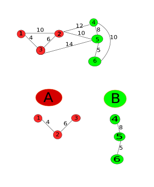
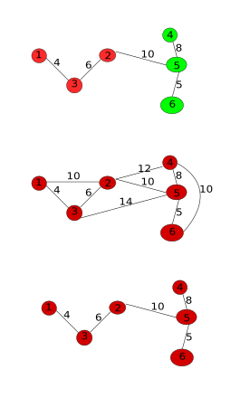
Note that the MSTMaxEdge represents the maximum edge for the minimum Spanning Tree which is actually the internal difference of the component. But where is Kruskal’s algorithm? Well, the edge causing the merge will be the maximum edge of the MST selected by kruskals algorithm:

We sort the edges and iterate through them in a non-descending order.
According to the algorithm, the difference between the components is the minimum edge weight $e_k$. And Int(C) is the maximum of the edge weights in the components ($e_i, e_j$). Remember that $e_i$ and $e_j$ are already iterated through because we iterating in a non-descending order and $e_i$ and $e_j$ are part of few components (Initially there is only one pixel in an image and therefore, no edges), which means $e_k > = e_i$ and $e_k > = e_j$
If the components are to be merged, a new component is to be created and therefore a new MST maximum edge. Creating the new MST is easy as we only need to connect the two MSTs (MSTs of the components) with the minimum edge(kruskals). This minimum edge is $e_k$ as established in the previous point.
As we know that $e_k$ is greater than maximum MST edges of the two components, $e_k$ becomes the new MSTMaxEdge.

The above shows a subset of the graph. The bottom image shows the MSTs of the two components. Component A's max edge is (2, 3) with weight 6 and Component B's max edge is (4, 5) with weight 8.

First image shows the edges considered by the algorithm and (2, 5) is the minimum edge connecting the two components. Second image shows, the graph when the components are merged into a single component. Third image shows that the max edge of the MST by kruskals algorithm in the merged component is the edge causing the merge, (2, 5) or the edge at the present iteration of the algorithm.

main.cpp

#include <iostream>
#include <vector>
#include <opencv2/opencv.hpp>
#include <string>
#include <filesystem>
#include "DisjointForest.h"
#include "utils.h"
#include "segmentation.h"

int main(int argc, char* argv[]) {
    if (argc != 7){
        std::cout << "Execute: .\\ImageSegment inputImage outputDir colorSpace k(float) sigma(float) minSize(int)\n";
        std::cout << "Exiting program\n";
        std::exit(1);
    }
    const std::string inputPath =  argv[1];
    const std::string outputFolder = argv[2];
    const std::string colorSpace = argv[3];

    float gaussianBlur, kValue;
    int minimumComponentSize;
    std::stringstream convert;

    convert << argv[4] << " " << argv[5] << " " << argv[6];
    if (!(convert >> kValue) || !(convert >> gaussianBlur) || !(convert >> minimumComponentSize)){
        std::cout << "Execute: .\\ImageSegment inputImage outputDir colorSpace k(float) sigma(float) minSize(int)\n";
        std::cout << "Something wrong with value k, sigma or minSize, (arguments - 5, 6, 7) \n";
        std::cout << "Exiting program\n";
        std::exit(1);
    }
    printParameters(inputPath, outputFolder, colorSpace, gaussianBlur, kValue, minimumComponentSize);

    const std::filesystem::path path = std::filesystem::u8path(inputPath);
    const std::string baseFileName = getFileNameFromPath(inputPath);
    std::cout << "Filename: " << baseFileName << '\n';

    std::srand(static_cast<unsigned int>(std::time(nullptr)));

    cv::Mat img = cv::imread(path, cv::IMREAD_COLOR);
    cv::GaussianBlur(img, img, cv::Size(3,3), gaussianBlur);
    const int rows = img.rows;
    const int columns = img.cols;
    std::cout << "Image Size:  " << img.size << '\n';

    std::vector<pixel_pointer> pixels = constructImagePixels(img, rows, columns);
    std::vector<edge_pointer> edges = setEdges(pixels, colorSpace, rows, columns);
    std::sort(edges.begin(), edges.end(), [] (const
    edge_pointer& e1, const edge_pointer& e2){
                                                        return e1->weight < e2->weight;
                                                        });

    int totalComponents = rows * columns;
    segmentImage(edges, totalComponents, minimumComponentSize, kValue);

    auto firstComponentStruct = pixels[0]->parentTree->parentComponentStruct;
    while(firstComponentStruct->previousComponentStruct){
        firstComponentStruct = firstComponentStruct->previousComponentStruct;
    }

    std::string outputPath = outputFolder + baseFileName + "-" + colorSpace + "-k" +
                             std::to_string(static_cast<int>(kValue)) + '-' + std::to_string(gaussianBlur) +"-"
                              "min" + std::to_string(static_cast<int>(minimumComponentSize)) + ".jpg";

    std::filesystem::path destinationPath = std::filesystem::u8path(outputPath);
    cv::Mat segmentedImage = addColorToSegmentation(firstComponentStruct, rows, columns);
    cv::imshow("Image", segmentedImage);
    cv::imwrite(destinationPath, segmentedImage);
    std::cout << "Image saved as: " << outputPath << '\n';
    cv::waitKey(0);

    return 0;
}

Explanation:

Operations of main.cpp in order:

Image is read into img, which is then smoothened with a Gaussian filter
Pixels and Edge Vectors are initialized
From the image, the Pixel objects are created, initialized and placed into pixels vector depending on the location of these pixels.
Edges are initialized and computed between neighbors as shown in the image above and placed into edges vector
The edges are sorted based on their weight
The segmentation algorithm is applied to the edges
The image is colored based on the segmentation results

Building and execution

You can run the following commands in any directory, but it is recommended to execute this in the same directory where source is located. Make sure cmake is installed.

mkdir build
cd build
cmake ../source
cmake --build .

Execute the program using the folling syntax from the build directory:

.\ImageSegment inputImage outputDir colorSpace k(float) sigma(float) minSize(int)\n";

Results

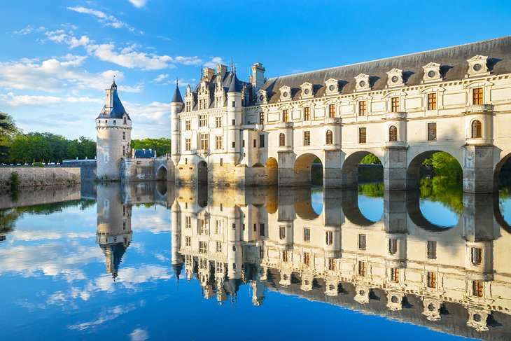
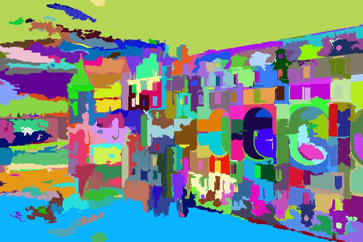
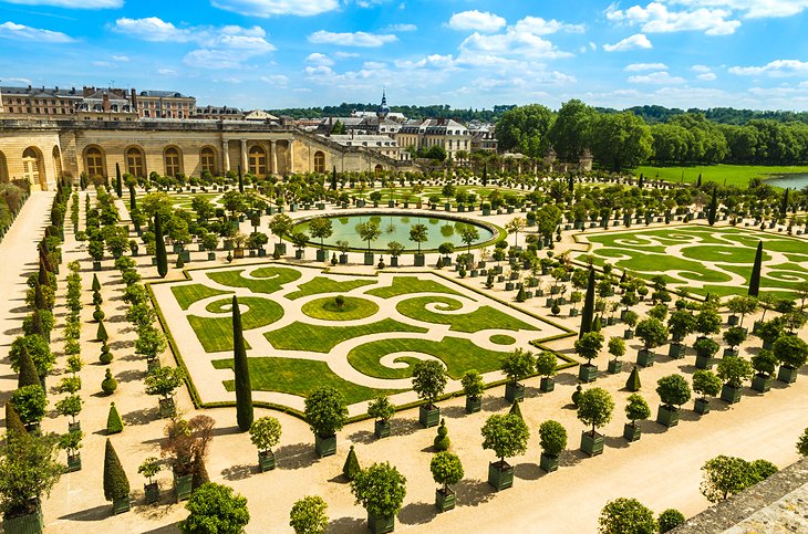
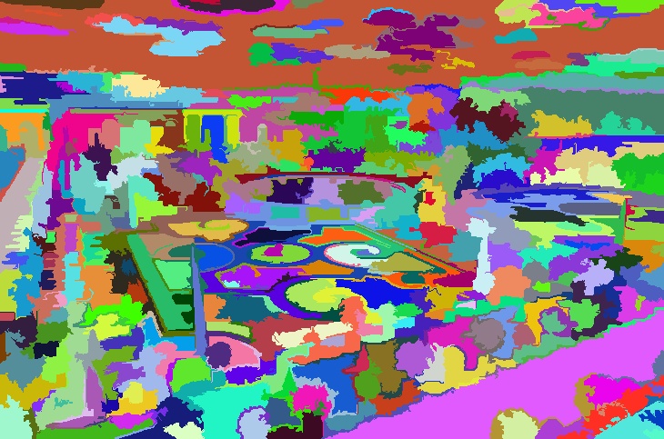
There is still some scope of improvement but this is a decent start.

Phew! We’re done. Don’t hesitate to contact me if you have any feedback or questions.

Written on June 3, 2020